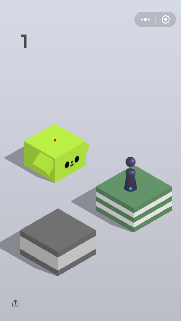
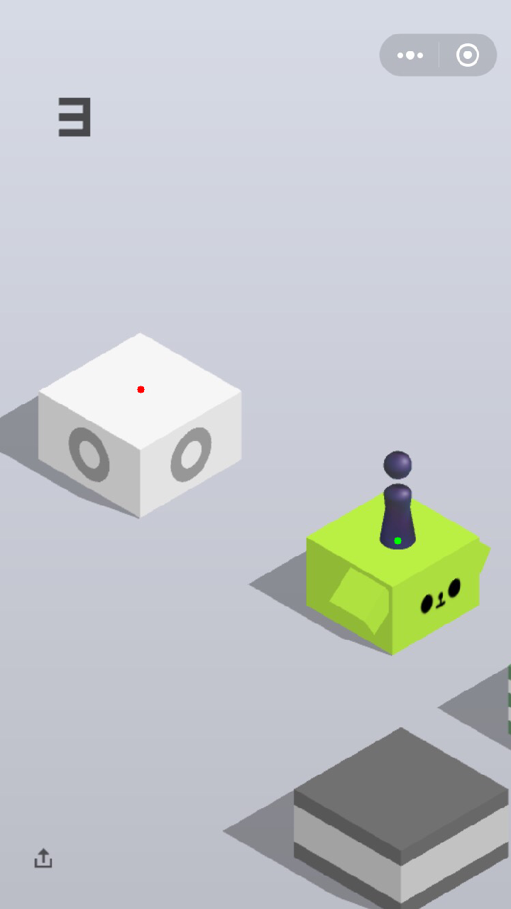
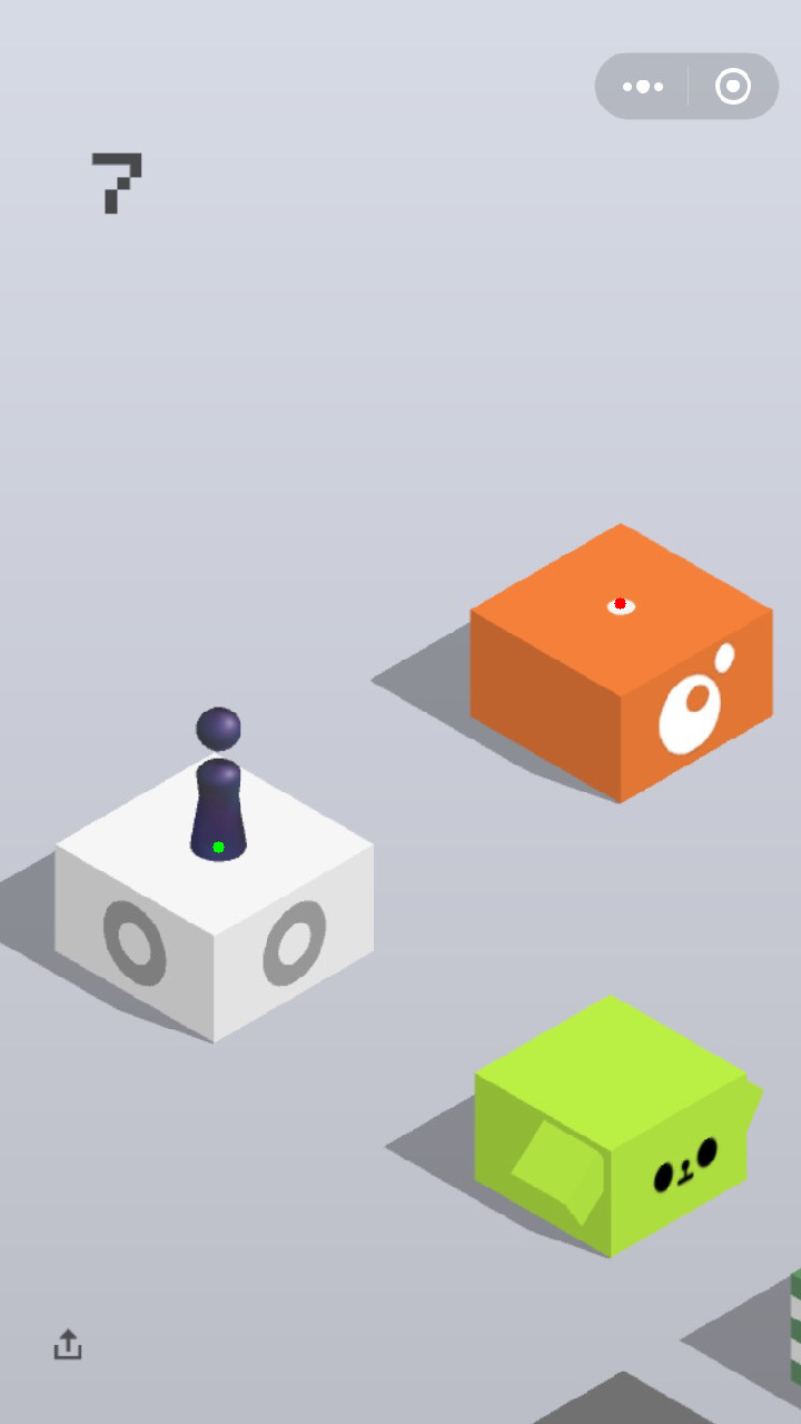
算法的第一步是获取手机屏幕的截图并可以控制手机的触控操作,我们的github仓库里详细介绍了针对Android和IOS手机的配置方法,你只需要按照将手机连接电脑,按照教程执行就可以完成配置。在获取到屏幕截图之后,就是个简单的视觉问题。我们需要找的就是小人的位置和下一次需要跳的台面的中心。 如图所示,绿色的点代表小人当前的位置,红点代表目标位置。


多尺度搜索(Multiscale Search)
这个问题可以有非常多的方法去解,为了糙快猛地刷上榜,我一开始用的方式是多尺度搜索。 我随便找了一张图,把小人抠出来,就像下面这样。

另外,我注意到小人在屏幕的不同位置,大小略有不同,所以我设计了多尺度的搜索,用不同大小的进行匹配, 最后选取置信度(confidence score)最高的。
多尺度搜索的代码长这样
def multi_scale_search(pivot, screen, range=0.3, num=10):
    H, W = screen.shape[:2]
    h, w = pivot.shape[:2]

    found = None
    for scale in np.linspace(1-range, 1+range, num)[::-1]:
        resized = cv2.resize(screen, (int(W * scale), int(H * scale)))
        r = W / float(resized.shape[1])
        if resized.shape[0] < h or resized.shape[1] < w:
            break
        res = cv2.matchTemplate(resized, pivot, cv2.TM_CCOEFF_NORMED)

        loc = np.where(res >= res.max())
        pos_h, pos_w = list(zip(*loc))[0]

        if found is None or res.max() > found[-1]:
            found = (pos_h, pos_w, r, res.max())

    if found is None: return (0,0,0,0,0)
    pos_h, pos_w, r, score = found
    start_h, start_w = int(pos_h * r), int(pos_w * r)
    end_h, end_w = int((pos_h + h) * r), int((pos_w + w) * r)
    return [start_h, start_w, end_h, end_w, score]
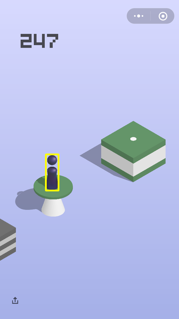
我们来试一试,效果还不错,应该说是又快又好,我所有的实验中找小人从来没有失误。 不过这里的位置框的底部中心并不是小人的位置,真实的位置是在那之上一些。
同理,目标台面也可以用这种办法搜索,但是我们需要收集一些不同的台面,有圆形的,方形的, 便利店,井盖,棱柱等等。由于数量一多,加上多尺度的原因,速度上会慢下来。这时候,我们就需要想办法加速了。 首先可以注意到目标位置始终在小人的位置的上面,所以可以操作的一点就是在找到小人位置之后把小人位置以下的 部分都舍弃掉,这样可以减少搜索空间。
但是这还是不够,我们需要进一步去挖掘游戏里的故事。小人和目标台面基本上是关于屏幕中心对称的位置的。 这提供了一个非常好的思路去缩小搜索空间。假设屏幕分辨率是(1280,720)的,小人底部的位置是(h1, w1), 那么关于中心对称点的位置就是(1280 - h1, 720 - w1),以这个点为中心的一个边长300的正方形内,我们再去多尺度搜索目标位置, 就会又快有准了。效果见下图,蓝色框是(300,300)的搜索区域,红色框是搜到的台面,矩形中心就是目标点的坐标了。
加速的奇技淫巧(Fast-Search)
玩游戏需要细心观察。我们可以发现,小人上一次如果跳到台面中心,那么下一次目标台面的中心会有一个白点,就像刚才 所展示的图里的。更加细心的人会发现,白点的RGB值是(245,245,245),这就让我找到了一个非常简单并且 高效的方式,就是直接去搜索这个白点,注意到白点是一个连通区域,像素值为(245,245,245)的像素个数稳定在 280-310之间,所以我们可以利用这个去直接找到目标的位置。这种方式只在前一次跳到中心的时候可以用,不过没有关系, 我们每次都可以试一试这个不花时间的方法,不行再考虑多尺度搜索。
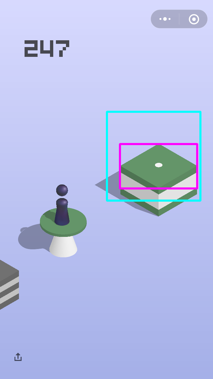
讲到这里,我们的方法已经可以运行的非常出色了,基本上是一个永动机。下面是用我的手机玩了一个半小时左右,跳了859次的状态, 我们的方法正确的计算出来了小人的位置和目标位置,不过我选择狗带了,因为手机卡的已经不行了。


这里有一个示例视频,欢迎观看!
到这里就结束了吗?那我们和业余玩家有什么区别?下面进入正经的学术时间,非战斗人员请迅速撤离!
CNN Coarse-to-Fine 模型
考虑到IOS设备由于屏幕抓取方案的限制(WebDriverAgent获得的截图经过了压缩,图像像素受损,不再是原来的像素值,原因不详,欢迎了解详情的小伙伴提出改进意见~)无法使用fast-search,同时为了兼容多分辨率设备,我们使用卷积神经网络构建了一个更快更鲁棒的目标检测模型,下面分数据采集与预处理,coarse模型,fine模型,cascade四部分介绍我们的算法。
数据采集与预处理
基于我们非常准确的multiscale-search、fast-search模型,我们采集了7次实验数据,共计大约3000张屏幕截图,每一张截图均带有目标位置标注,对于每一张图,我们进行了两种不同的预处理方式,并分别用于训练coarse模型和fine模型,下面分别介绍两种不同的预处理方式。
coarse 模型数据预处理
由于每一张图像中真正对于当前判断有意义的区域只在屏幕中央位置,即人和目标物体所在的位置,因此,每一张截图的上下两部分都是没有意义的,因此,我们将采集到的大小为(1280, 720)的图像沿h方向上下各截去(320, 720)大小,只保留中心(640, 720)的图像作为训练数据。
我们观察到,游戏中,每一次当小人落在目标物中心位置时,下一个目标物的中心会出现一个白色的圆点,
考虑到训练数据中fast-search会产生大量有白点的数据,为了杜绝白色圆点对网络训练的干扰,我们对每一张图进行了去白点操作,具体做法是,用白点周围的纯色像素填充白点区域。
fine 模型数据预处理
为了进一步提升模型的精度,我们为fine模型建立了数据集,对训练集中的每一张图,在目标点附近截取320*320大小的一块作为训练数据,

为了防止网络学到trivial的结果,我们对每一张图增加了50像素的随机偏移。fine模型数据同样进行了去白点操作。
coarse 模型
我们把这一问题看成了回归问题,coarse模型使用一个卷积神经网络回归目标的位置,
def forward(self, img, is_training, keep_prob, name='coarse'):
    with tf.name_scope(name):
        with tf.variable_scope(name):
            out = self.conv2d('conv1', img, [3, 3, self.input_channle, 16], 2)
            # out = tf.layers.batch_normalization(out, name='bn1', training=is_training)
            out = tf.nn.relu(out, name='relu1')

            out = self.make_conv_bn_relu('conv2', out, [3, 3, 16, 32], 1, is_training)
            out = tf.nn.max_pool(out, [1, 2, 2, 1], [1, 2, 2, 1], padding='SAME')

            out = self.make_conv_bn_relu('conv3', out, [5, 5, 32, 64], 1, is_training)
            out = tf.nn.max_pool(out, [1, 2, 2, 1], [1, 2, 2, 1], padding='SAME')

            out = self.make_conv_bn_relu('conv4', out, [7, 7, 64, 128], 1, is_training)
            out = tf.nn.max_pool(out, [1, 2, 2, 1], [1, 2, 2, 1], padding='SAME')

            out = self.make_conv_bn_relu('conv5', out, [9, 9, 128, 256], 1, is_training)
            out = tf.nn.max_pool(out, [1, 2, 2, 1], [1, 2, 2, 1], padding='SAME')

            out = tf.reshape(out, [-1, 256 * 20 * 23])
            out = self.make_fc('fc1', out, [256 * 20 * 23, 256], keep_prob)
            out = self.make_fc('fc2', out, [256, 2], keep_prob)

    return out
经过十小时的训练,coarse模型在测试集上达到了6像素的精度,实际测试精度大约为10像素,在测试机器(MacBook Pro Retina, 15-inch, Mid 2015, 2.2 GHz Intel Core i7)上inference时间0.4秒。这一模型可以很轻松的拿到超过1k的分数,这已经远远超过了人类水平和绝大多数自动算法的水平,日常娱乐完全够用,不过,你认为我们就此为止那就大错特错了~
fine 模型
fine模型结构与coarse模型类似,参数量稍大,fine模型作为对coarse模型的refine操作,
def forward(self, img, is_training, keep_prob, name='fine'):
    with tf.name_scope(name):
        with tf.variable_scope(name):
            out = self.conv2d('conv1', img, [3, 3, self.input_channle, 16], 2)
            # out = tf.layers.batch_normalization(out, name='bn1', training=is_training)
            out = tf.nn.relu(out, name='relu1')

            out = self.make_conv_bn_relu('conv2', out, [3, 3, 16, 64], 1, is_training)
            out = tf.nn.max_pool(out, [1, 2, 2, 1], [1, 2, 2, 1], padding='SAME')

            out = self.make_conv_bn_relu('conv3', out, [5, 5, 64, 128], 1, is_training)
            out = tf.nn.max_pool(out, [1, 2, 2, 1], [1, 2, 2, 1], padding='SAME')

            out = self.make_conv_bn_relu('conv4', out, [7, 7, 128, 256], 1, is_training)
            out = tf.nn.max_pool(out, [1, 2, 2, 1], [1, 2, 2, 1], padding='SAME')

            out = self.make_conv_bn_relu('conv5', out, [9, 9, 256, 512], 1, is_training)
            out = tf.nn.max_pool(out, [1, 2, 2, 1], [1, 2, 2, 1], padding='SAME')

            out = tf.reshape(out, [-1, 512 * 10 * 10])
            out = self.make_fc('fc1', out, [512 * 10 * 10, 512], keep_prob)
            out = self.make_fc('fc2', out, [512, 2], keep_prob)

    return out
经过十小时训练,fine模型测试集精度达到了0.5像素,实际测试精度大约为1像素,在测试机器上的inference时间0.2秒。
cascade
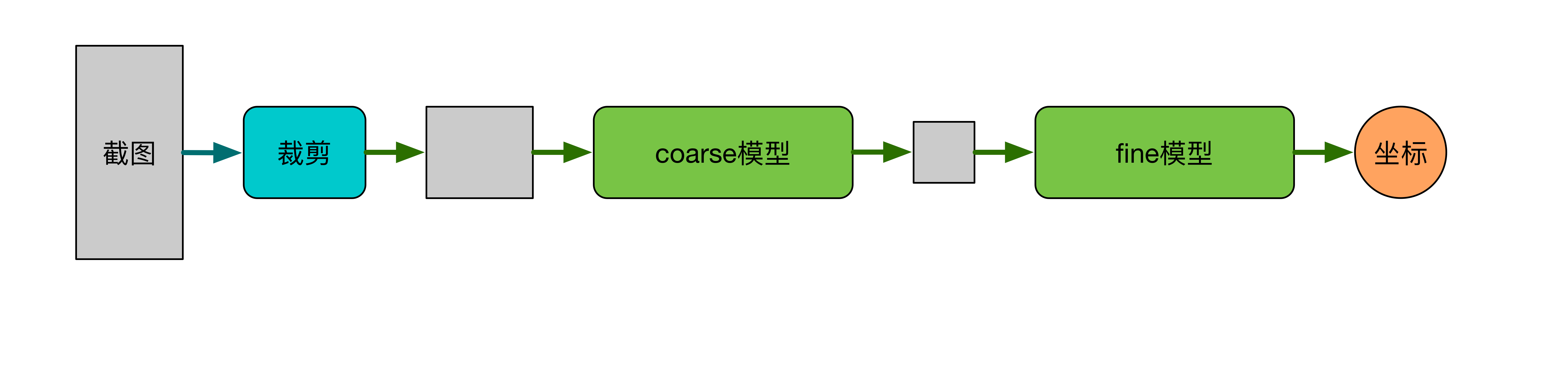
总体精度1像素左右,时间0.6秒。
总结
针对这一问题,我们利用AI和CV技术,提出了合适适用于IOS和Android设备的完整解决方案,稍有技术背景的用户都可以实现成功配置、运行,我们提出了Multiscale-Search,Fast-Search,CNN Coarse-to-Fine三种解决这一问题的算法,三种算法相互配合,可以实现快速准确的搜索、跳跃,用户针对自己的设备稍加调整跳跃参数即可接近实现“永动机”。讲到这里,似乎可以宣布,我们的工作terminate了这个问题,微信小游戏跳一跳game over!
友情提示:适度游戏益脑,沉迷游戏伤身,技术手段的乐趣在于技术本身而不在游戏排名,希望大家理性对待游戏排名和本文提出的技术,用游戏娱乐自己的生活
声明:本文提出的算法及开源代码符合MIT开源协议,以商业目的使用该算法造成的一切后果须由使用者本人承担
Contributors
- Xiao Taihong xiaotaihong@126.com
- An Jie jie.an@pku.edu.cn