An Overview on Optimization Algorithms in Deep Learning 2
Published:
In the last article, I have introduced several basic optimization algorithms. However, those algorithms rely on the hyperparameter - the learning rate $\eta$ that has a significant impact on model performance. Though the use of momentum can go some way to alleviate these issues, it does so by introducing another hyperparameter $\rho$ that may be just as difficult to set as the original learning rate. In the face of this, it’s naturally to find other way to set learning rate automatically.
AdaGrad
AdaGrad algorithm adapts the learning rates of all model parameters by scaling them inversely proportional to the accumulated sum of squared partial derivatives over all training iterations. The update rule for AdaGrad is as follows:
\[\Delta \theta = -{\eta\over \sqrt{\sum_{\tau=1}^t g_{\tau}^2}}g_t\]Here the denominator computes the $l^2$ norm of all previous gradients on a per-dimension basis and $\eta$ is a global learning rate shared by all dimensions.
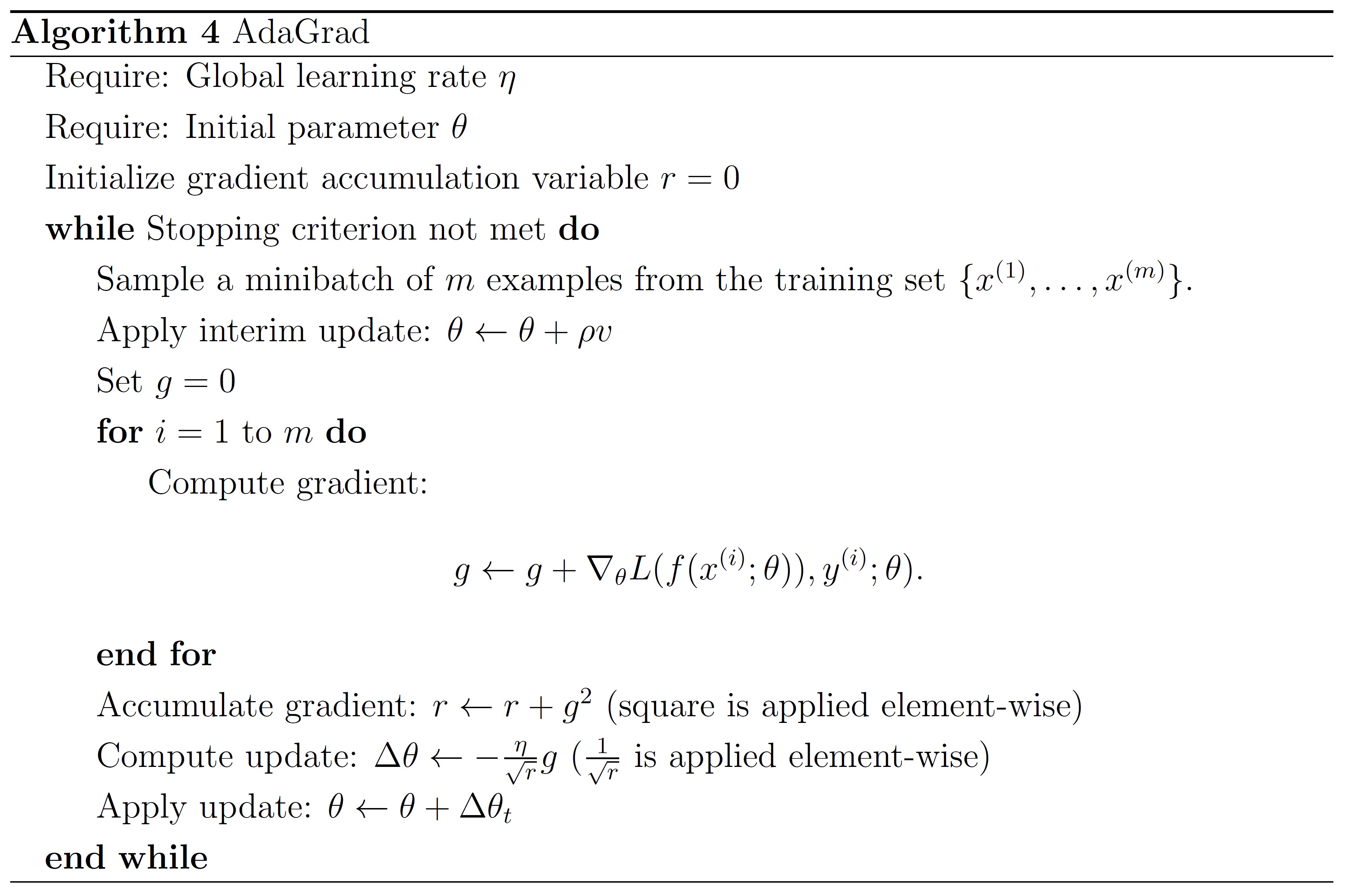
The AdaGrad algorithm relies on the first order information but has some properties of second order methods and annealing. Since the dynamic rate grows with the inverse of gradient magnitudes, large gradients have smaller learning rates and small gradients have large learning rates. This nice property, as in second order methods, makes progress along each dimension even out over time. This is very useful in deep learning model, because the scale of gradients in each layer varies by several orders of magnitude. Additionally, the denominator of the scaling coefficient has the same effects as annealing, reducing the learning rate over time.
RMSprop
The RMSprop algorithm addresses the deficiency of AdaGrad by changing the gradient accumulation into an exponentially weighted moving average. In deep networks, directions in parameter space with strong partial derivatives may flatten out early, so RMSprop introduces a new hyperparameter $\rho$ that controls the length scale of the moving average to prevent that from happening.
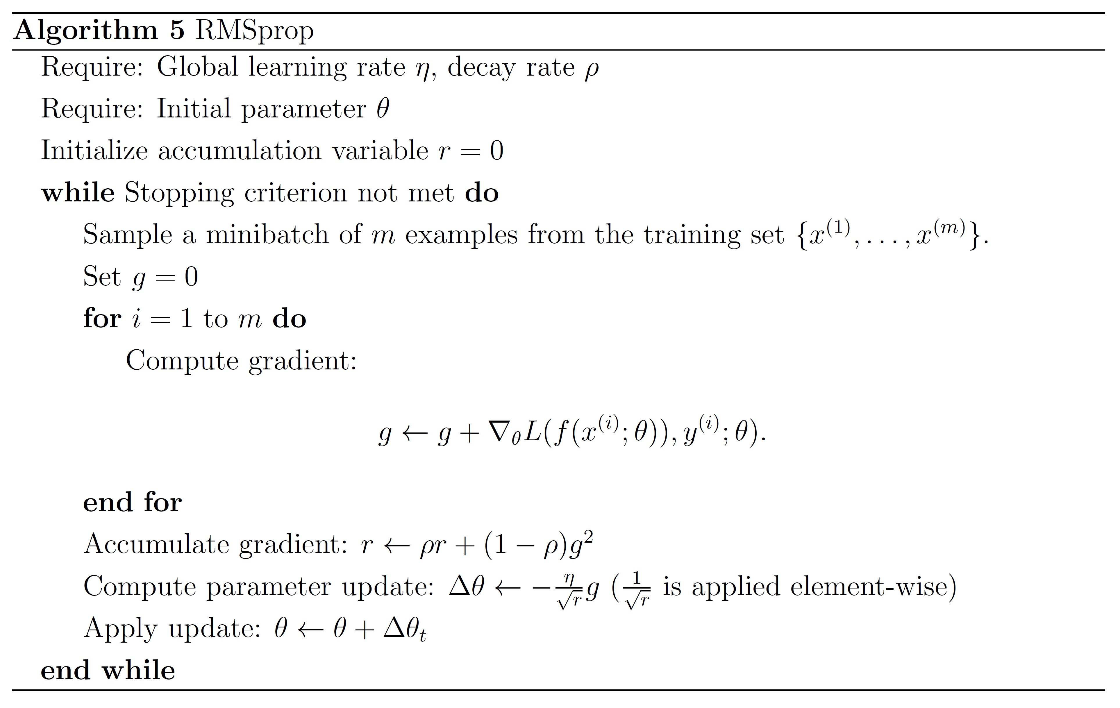
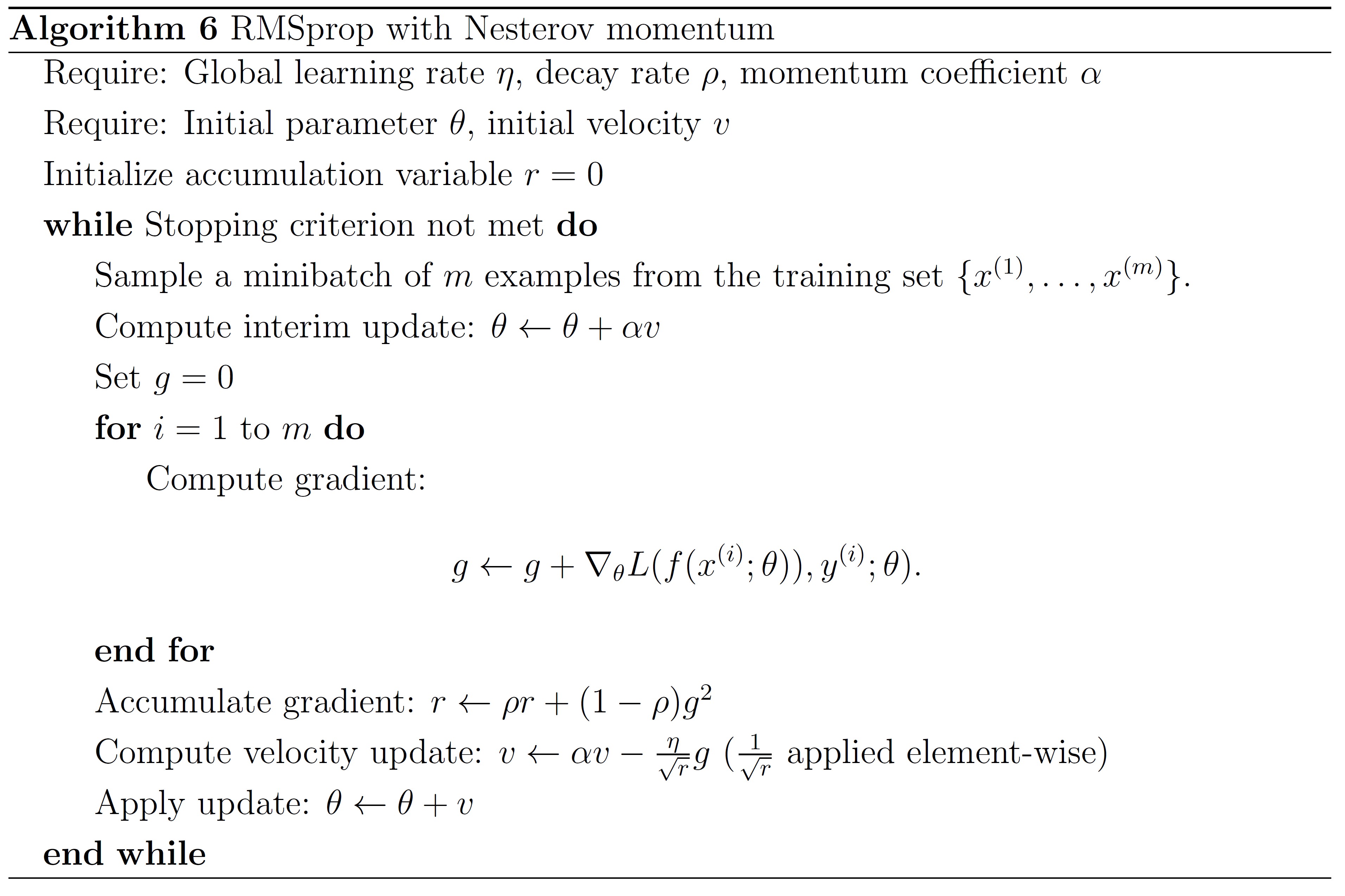
RMSprop with Nesterov momentum algorithm is shown below.
Adam
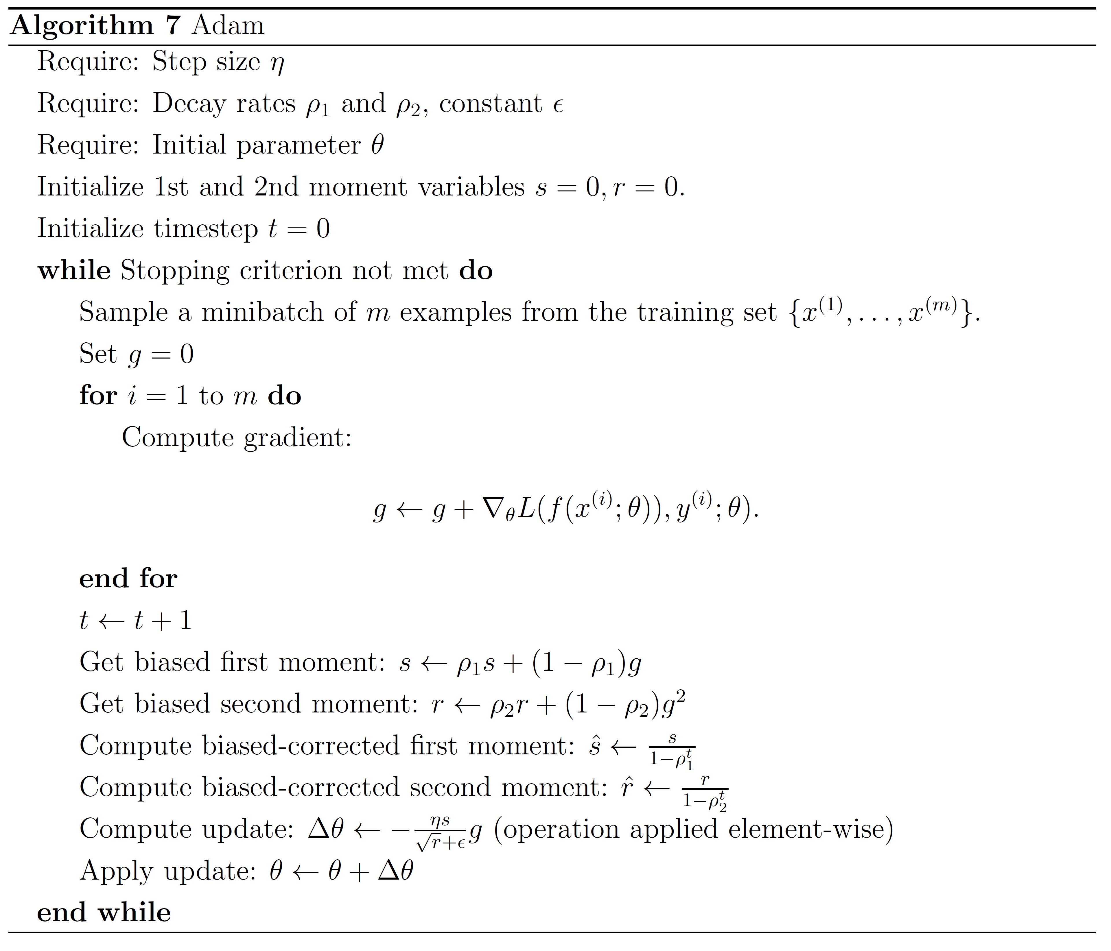
Adam is another adaptive learning rate algorithm presented below. It can been seen as a combination of RMSprop and momentum. Adam algorithm includes bias corrections to the estimates of both the first order moment and second order moment to prevent parameters from high bias early in training.
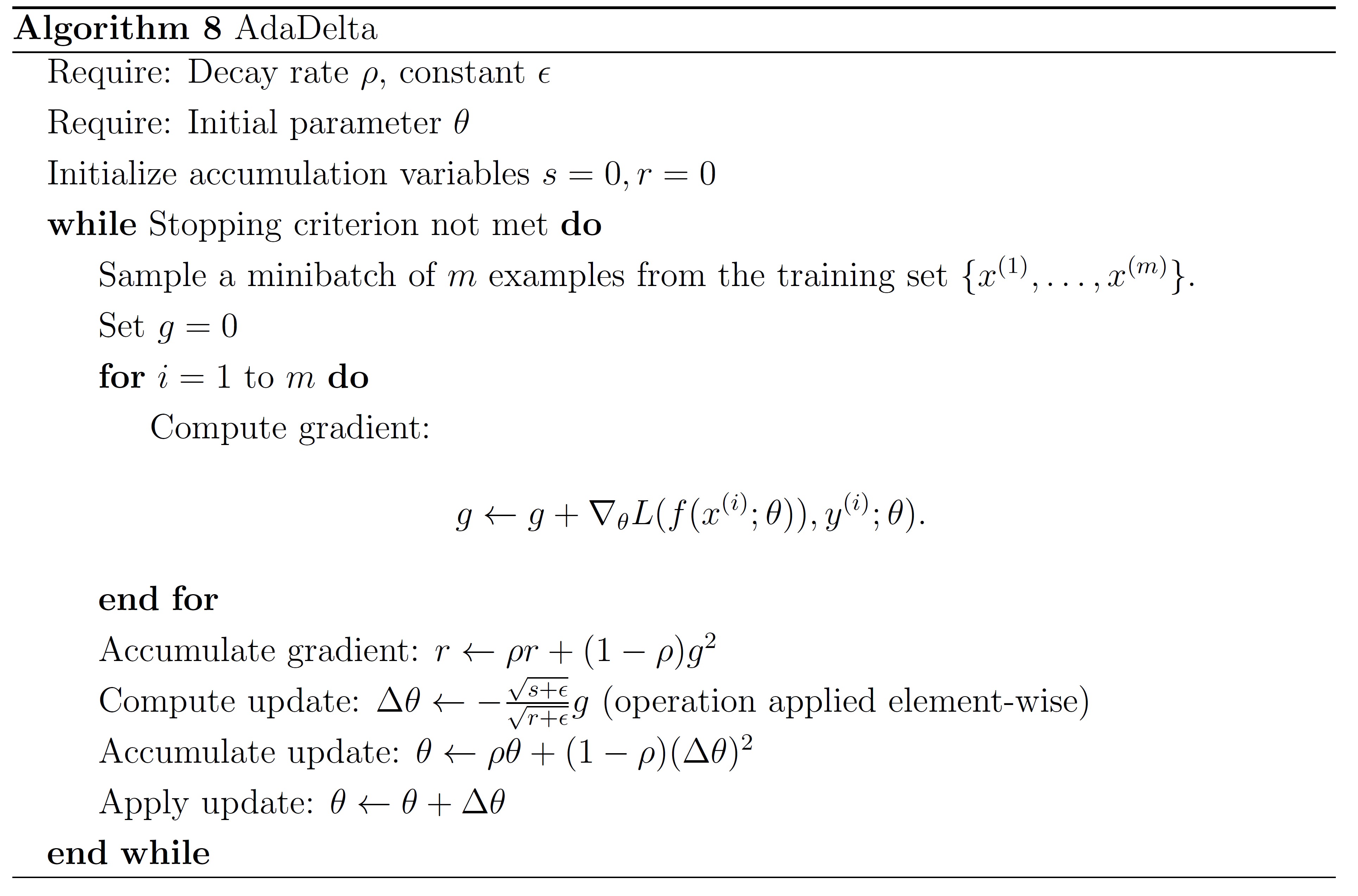
AdaDelta
This method was derived from AdaGrad in order to improve upon the two main drawbacks of the method:
- the continual decay of learning rates throughout training;
- the need for a manually selected global learning rate.
Instead of accumulating the sum of squared gradients over all time, we restricted the window of past gradients that are accumulated to be some fixed size $w$ instead of size $t$ where $t$ is the current iteration as in AdaGrad. Since storing $w$ previous squared gradients is inefficient, our methods implements this accumulation as an exponentially decaying average of the squared gradients. Assume at time $t$ this running average is $\E(g^2)_t$ then we compute
\[\E(g^2)_t = \rho \E(g^2)_{t-1} +(1-\rho)g_t^2\]Since we require the square root of this quantity in the parameter updates, this effectively becomes the RMS of previous squared gradients up to time $t$
\[\RMS(g)_t=\sqrt{\E(g^2)_t+\epsilon}\]The resulting parameter update is then
\[\Delta\theta = -{\eta\over \RMS(g)_t}g_t \tag 1\label{eq-1}\]Since the RMS of the previous gradients is already presented in the denominator in \eqref{eq-1}, we considered a measure of the $\Delta\theta$ quantity in the numerator. By computing the exponentially decaying RMS over a window of size $w$ of previous $\Delta\theta$ to give the AdaDelta method:
\[\Delta\theta=-{\RMS(\Delta\theta)_{t-1}\over \RMS(g)_t}g_t\]where the same constant $\epsilon$ is added to the numerator RMS as well to ensure progress continues to be made even if previous updates becomes small.
Extra boon: A pdf-format cheet sheet containing all these algorithms could be downloaded here for reference.
